Distillation Tutorial V: Azeotropes and Distillation Boundaries (Main Page)
Some mixtures can have very peculiar phase behavior where a specific composition of the mixture behaves as if it were a pure component (i.e. its bubble and dew points are the same) and where the definition of light and heavy component changes over different composition ranges. Such mixtures are called azeotropic mixtures and as we will show you in this tutorial, they can place limits on the separations that can be made. In this tutorial, you will learn about
- Azeotropes and azeotropic mixtures.
- Distillation boundaries.
- The role of azeotropes and distillation boundaries in distillation design.
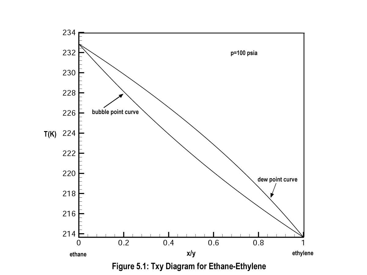
5.1 Introduction.If you go back to Tutorial I and look at the Txy diagrams for some of the binary mixtures studied, you will notice that the only places where the bubble point and dew point curves meet are at the pure component ends. Here x = y = 0 or x = y = 1 and this means that pure components have a boiling point or change phase at constant temperature when the pressure is fixed. For example, for the ethane-ethylene Txy diagram shown in Fig. 5.1, you clearly see that the bubble and dew point curves meet at x (ethylene) = y (ethylene) = 0 and x (ethylene) = y (ethylene) = 1.
Just press play.
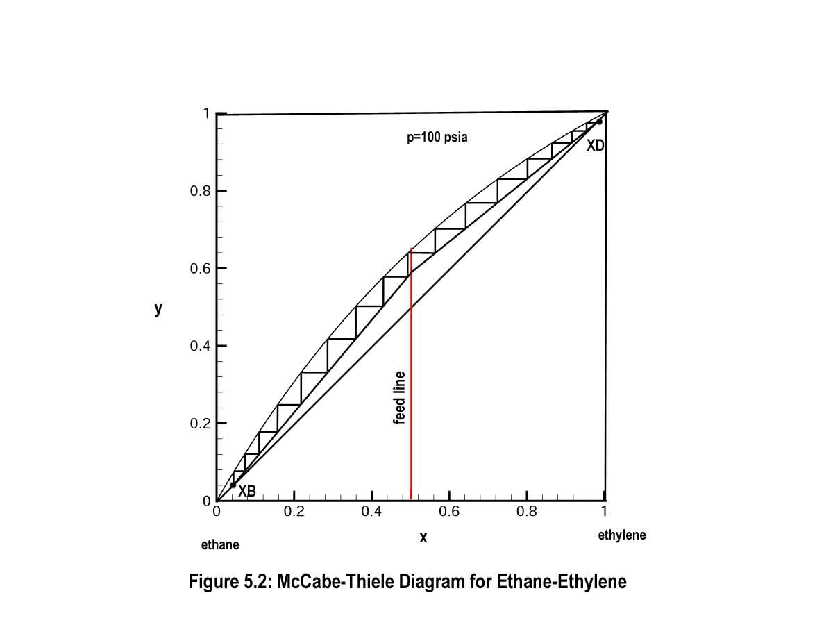
This is direct consequence of the phase behavior of ethylene and ethane. Mixtures of these species behave according to Raoult's law and show very simple phase behavior. The corresponding yx diagram for ethylene and ethane is equally simple and quite useful in the McCabe-Thiele distillation design procedure. This yx diagram and corresponding McCabe-Thiele plot are shown in Fig. 5.2. Notice that the yx diagram forms a nice arch-like curve that runs from one pure component end to the other.
Just press play.
However, not all mixtures behave like ethylene and ethane. Some, like acetone and water, show more complex behavior where the yx curve changes its shape dramatically over the composition range from 0 to 1. This kind of behavior and its consequence of a tangent pinch point are shown in Fig. 5.3.
Just press play.
For mixtures like acetone and water, Raoult's law is not sufficient to describe the vapor-liquid equilibrium and more complicated models are generally used. However, despite this more complicated phase behavior, the only place where y = x is at the pure component ends.
5.2 Binary Azeotropic Mixtures. A binary azeotropic mixture is a mixture whose yx curve crosses the 45-degree line somewhere between x > 0 and x < 1. The point at which this occurs is called an azeotropic point and it is defined mathematically by the simple equation y = x. Figure 5.4 is an example of a mixture that shows azeotropic behavior – chloroform and acetone.
Just press play.
The azeotropic point for chloroform-acetone is at approximately x (chloroform) = y (chloroform) = 0.64. Figure 5.4 also shows you that to the left of the azeotropic point, the yx curve is below the 45-degree line and to the right of the azeotropic point, the yx curve is above the 45-degree line and behaves more like what you are used to seeing. When the yx curve is below the 45-degree line, it says that chloroform is actually the heavy component and acetone is the light component. This means the K-value for chloroform is less than 1 and the K-value for acetone is greater than 1 in this region. On the right side of Fig. 5.4, chloroform is the light component and acetone is the heavy component – so the relative magnitude of the K-values is reversed. That is, to the right side of the azeotropic point in Fig. 5.4, the K-value of chloroform is greater than 1 and the K-value of acetone is less than 1. Strange, don't you think? Actually, this type of mixture behavior, called azeotropic behavior, is more common than you might imagine.
Figure 5.5 shows the Txy diagram for chloroform and acetone at atmospheric pressure. The first thing that you should notice is that the Txy diagram is also divided into two parts – just like the yx diagram in Fig. 5.4. To the left, the temperature rises from the boiling point of acetone to a maximum at T = 339.12 K at the azeotropic point. To the right, the temperature decreases from the azeotropic point to the boiling point of chloroform. Since the azeotropic point has the highest boiling point (i.e. bubble or dew point) of any composition between x = 0 and x = 1, this type of azeotrope is called a maximum boiling azeotrope. There are also binary mixtures whose azeotropic temperatures correspond to the lowest temperature of any composition betweeen 0 and 1 and these azeotropes are called minimum boiling azeotropes. Ethanol and water at atmospheric pressure is an example of a mixture that has a minimum boiling azeotrope.
Just press play.
Figures 5.3 and 5.4 show that binary azeotropes create a 'boundary' that cannot be crossed by distillation. By this we mean that if the feed composition is to the left of the azeotropic point, then both products must also lie to the left of the azeotropic point. The same is true for the feed composititons to the right of the azeotropic point. Feed compositions to the right of the azeotropic point require that the products are also to the right of the azeotropic point. See Figs. 5.3 and 5.4.
Practice Exercises. Please answer the following using the programs I will give you.
- Determine the Txy and yx diagrams for ethanol and water at atmospheric pressure.
- What is the azeotropic composition?
- What is the azeotropic temperature?
- What are the K-values of ethanol and water at the azeotropic point?
- Explain why your answer to question 4 makes physical sense.
- Perform a McCabe-Thiele analysis with a bottoms product specification to the left of the azeotropic composition and a distillate product composition to the right of the azeotropic point. Let the feed be any composition between the bottoms and distillate compositions you select. Explain clearly what difficulties you run into.
- For feed compositions to the left of the azeotrope, what is the highest distillate composition of ethanol that can be achieved? Why?
- For feed compositions to the right of the azeotrope, what is the lowest bottoms composition of ethanol that can be achieved? Why?
- What do your answers to questions 7 and 8 say about the possible consequences caused by azeotropes on achievable separations? Why?
5.3 Ternary Azeotropic Mixtures. Azeotropic behavior and its consequences are not limited to binary mixtures. A mixture with any number of components can have azeotropes and the complexities only increase as the number of components increases. For example, the ternary mixture of chloroform, acetone and benzene at atmospheric pressure has one binary azeotrope between chloroform and acetone as shown in Fig. 5.6. Notice that this azeotrope gives rise to an interior distillation boundary (shown in blue) that runs from the benzene corner or vertex to the chloroform-acetone azeotrope.
Just press play.
Also notice that the trajectories for the distillation lines in Fig. 5.6 show that boundaries in ternary mixtures can be crossed! Look closely in the area around the bottoms product composition. These distillation lines actually start in the region below the blue boundary curve and extend into the region above the blue curve. However, boundaries in ternary mixtures can only be crossed from the side that bulges toward the distillation line (called concave side) and generally the starting point of the distillation line (i.e. in this case the bottoms product composition) must be fairly close to the boundary for this to happen.
Some mixtures, like chloroform, methanol, and acetone, have even more complicated behavior. In particular, chloroform (1), methanol (2), and acetone (3) at atmospheric pressure has four azeotropes – three binary azeotropes and one ternary azeotrope. The azeotropic compositions and temperatures are shown in the table below.
| Azeotrope | (x1, x2, x3) | Temperature (K) |
| 1 | (0.6531, 0.3469, 0) | 327.52 |
| 2 | (0.6414, 0, 0.3586) | 339.12 |
| 3 | (0, 0.2343, 0.7657) | 329.74 |
| 4 | (0.2173, 0.4470, 0.3357) | 331.71 |
Figure 5.7 shows the azeotropes for this mixture along with the distillation boundaries. Note that there are four distinct distillation regions.
Just press play.
Quick Exercise. Find the boiling points of chloroform, methanol and acetone and determine whether the azeotropes given in the table are maximum boiling, minimum boiling, or saddle point (i.e. above one boiling point, but below the other) azeotropes.
5.4 Approximating Distillation Boundaries. Since boundaries caused by azeotropes can place limitations on the separations that can be made by distillation, it is often important to be able to compute the location of these boundaries as part of the design process. In this section, we show you how to generate approximate boundaries using distillation lines at total reflux.
Generating approximate distillation boundaries is a relatively straightforward procedure that requires the use of either the rectifying or stripping line equation at total reflux. Therefore, consider either Eq. 4.1 or 4.2 from Tutorial IV.
| xj+1 = [s / (s + 1)] yj - [1 / (s + 1)] xB | (5.1) |
| xj+1 = [(r + 1) / r] yj + [1 / r] xD | (5.2) |
At total reboil or reflux, these equations become very simple
| xj+1 = yj | (5.3) |
Quick Exercise. Show that Eqs. 5.1 or 5.2 reduces to Eq. 5.3 at total reboil or total reflux, respectively.
The procedure for finding a distillation boundary is as follows.
- Choose a very high value of reflux ratio or stripping ratio. I typically use 1 x 10200.
- Systematically select a value of xB = x1 (composition on stage 1 or reboiler) very, very close to the high boiling component.
- Use a bubble point calculation to calculate y1 and apply Eq. 5.3. and find x2.
- Repeat step 3, finding in turn x3, x4, ..., xN until your calculations go outside the composition triangle or they reach a light boiling component. The sequence of values {x1, x2, x3, ..., xN} is called a trajectory. Also remember that this light boiling component could actually be a minimum boiling azeotrope. Measure the total distance from x1 to xN.
- Repeat steps 2 and 3 for a large number of values of xB = x1. The boundary is the trajectory of largest distance.
Let's go through the process of generating an approximate distillation boundary for chloroform, acetone, and benzene at atmospheric pressure.
- Set r or s = 1 x 10200.
- Select z = 0.
- Calculate θ = (πz)/2. The value of q will be in radians.
- Pick (x1, x2) = (0, 0) + 1. x 10-03[cosθ, sinθ]. What this does is place an estimate of some bottoms composition close to the benzene vertex.
- Calculate the distillation line for this value of θ and record the distance. (For z = 0 you should get a distance of D = 1.)
- Choose the following sequence of z values - {z} = {2. x 10-07, 3.3 x 10-07, 3.7 x 10-07, 3.9 x 10-07, 4. x 10-07, 6. x 10-07, 1. x 10-06, 5. x 10-06, 1.} - and repeat steps 3, 4 and 5 for all z.
Performing these calculations and plotting the results you should get a figure very much like Fig. 5.8, where the portion of the red curve that runs from the benzene vertex to a neighborhood of the azeotrope represents an approximation to the true boundary (i.e. the blue curve). It is also important to understand that the accuracy of the approximation to any boundary depends, in part, on how accurately the variable z (or the angle θ) is estimated. Finally, note that the trajectories flow from high temperature (i.e. the benzene vertex) to one of two different lower boiling components (i.e. the chloroform vertex and the acetone vertex) and the approximation of the distillation boundary is the trajectory that has the locally longest distance in each distillation region.
Just press play.
Quick Exercise. The value of z that gives the approximation of the distillation boundary in Fig. 5.8 is z = 4 x 10-07. See if you can get a more accurate approximation to the boundary by estimating the variable z, which must lie between 3.9 x 10-07 and 4 x 10-07 to more significant digits.
Practice Exercise. Determine approximate distillation boundaries for chloroform, methanol and acetone at 1 atm by
- Generating five (5) trajectories from the highest boiling component and any maximum boiling azeotrope in the system. Pay particular attention to this point so that your trajectories flow from high temperature to low temperature in each suspected distillation region. Also pay attention to where the trajectories end. They should end at a low boiling component or minimum boiling azeotrope.
- Record the distance of each trajectory.
- Plot your results for all trajectories and see how closely or poorly the boundaries that you have calculated approximate the true distillation boundaries shown in Fig. 5.7.
- Verify that the locally longest distillation line in each region defines the boundary.
Summary Exercise. Please do the following.
- Generate trajectories and distillation boundaries for ethanol (1), benzene (2), and water (3) at 1 atm.
- Determine any azeotropes by carefully selecting other trajectories.
- Plot trajectories, distillation boundaries, and azeotropes on a triangular diagram.
- What does your plot tell you about the feasibility of designing a distillation column that produces denatured (or very high purity) ethanol at the bottom of the column - say xB (ethanol) = 0.999?
- What is a reasonable distillate product for this column?
- In practice such a column has two feeds - the near azeotropic mixture of ethanol and water that is fed high in the column, and a mixture of ethanol, benzene, and water that is fed on the top stage in the column. Suggest modifications of the stripping and rectifying line equations to handle two feed columns.
- Design a distillation column that produces denatured ethanol as the bottoms product.
- Find the minimum energy requirements for your distillation column design.